Coalition analysis (KOALA) 2017German election coalition probabilitiesAlexander Bauer | Andreas BenderStaBLab, LMU München2017/09/201 / 42

OutlineMotivation
2 / 42

Outline

Motivation
Implementation (Backend)

2 / 42

Outline

Motivation
Implementation (Backend)
Implementation (Frontend)

2 / 42

Outline

Motivation
Implementation (Backend)
Implementation (Frontend)
Outlook & sources

2 / 42

Motivation

When covering the election, media outlets (TV and print) mostly focus on questions like

Which parties will pass the 5% threshold and enter the "Bundestag" (German parliament)?

and

Which parties will form the governing coalition (currently Union - SPD, so called grand coalition)?

For the 2017 election also of special interest

Which party will have the 3rd largest share of votes?

3 / 42

Motivation

To answer these questions, pundits and writers usually focus on raw voting intention polls:

"Which party would you vote for if election was today?"

Last FORSA poll before the 2013 election (September, 20th); n = 1995
Union	SPD	Greens	FDP	The Left	Pirates	AfD	Others
40%	26%	10%	5%	9%	2%	4%	4%

4 / 42

Motivation

Interpretation of raw polls is problematic for several reasons

Sample uncertainty is ignored (even if the sample is representative, we would expect individual polls to deviate from the true shares).
- Exhibit 1.a: pollytix - Koalitionsrechner
- Exhibit 1.b: Tagesschau
Redistribution of votes is ignored (all votes for parties that do not pass the 5% threshold are redistributed proportionally to parties that pass the threshold).
- Exhibit 2: FAZ
Overreaction to individual polls (Some polls can be "off" or only depict the voting intention in a very short time-period; different weighting methods used by different pollsters)
- see Exhibits 1.b and 2

5 / 42

Example: BTW13

Last FORSA poll before the 2013 election (September, 20th); n = 1995
Union	SPD	Greens	FDP	The Left	Pirates	AfD	Others
40%	26%	10%	5%	9%	2%	4%	4%

6 / 42

Example: BTW13

Taking this poll at face value, 10% of votes would be redistributed:

Union	SPD	Greens	FDP	The Left
44.44%	28.89%	11.11%	5.56%	10%

7 / 42

Example: BTW13

This still ignores the sample uncertainty
Therefore, we sample election outcomes from the Dirichlet distribution

forsa_13$percent
round(gtools::rdirichlet(3, 1995*forsa_13$percent+0.5), 4)

##        [,1]   [,2]   [,3]   [,4]   [,5]   [,6]   [,7]   [,8]
## [1,] 0.4022 0.2634 0.1014 0.0439 0.0894 0.0157 0.0425 0.0414
## [2,] 0.4206 0.2526 0.0915 0.0446 0.0949 0.0210 0.0336 0.0413
## [3,] 0.4152 0.2629 0.0965 0.0518 0.0872 0.0154 0.0356 0.0353

round(gtools::rdirichlet(3, 20*forsa_13$percent+0.5), 4)

##        [,1]   [,2]   [,3]   [,4]   [,5]   [,6]   [,7]   [,8]
## [1,] 0.4861 0.2415 0.0551 0.0123 0.0663 0.0148 0.0969 0.0270
## [2,] 0.2443 0.1557 0.2510 0.1100 0.0548 0.0205 0.0898 0.0738
## [3,] 0.4347 0.2295 0.0750 0.1335 0.0505 0.0016 0.0732 0.0021

8 / 42

Example: BTW13

Based on a simulation with $n = 10000$ , FDP would not pass the 5% threshold in 50% of the cases
This leads to a bimodal distribution (after redistribution)

9 / 42

Example: BTW13

Coalition probabilities can be obtained by calculating the area underneath the probability distribution for $x > 50$
Or simpler: $P (event | sample) = \frac{# simulations with event}{# simulations}$

10 / 42

KOALA: Coalitions Analysis

In our approach we

aggregate polls from different pollsters within a 14-day time-window (pooled survey)
Calculate the Posterior Dirichlet distribution (based on Multinomial Likelihood and flat/uninformative Dirichlet Prior)
Calculate "secondary" properties (e.g. probability that Union-FDP would have simple majority) via Monte-Carlo sampling
- Simulate election outcomes from known Posterior (based on current pooled survey)
- $P (event | s a m p l e) = \frac{# event}{number of simulations}$

11 / 42

Implementation (Backend)

Backend implemented in the R-package coalitions (see Workflow vignette)
- scrapes wahlrecht.de for (new) polls
- (calculates pooled sample)
- calculate and sample from Posteriori
- Redistribute votes below 5% threshold and calculate Seats based on method by Sainte-Lague-Scheppers (German Law)
- Calculate coalition probabilities

12 / 42

Implementation (Backend)

Install via

devtools::install_github("adibender/coalitions")

Surveys returned as nested tidy data set (tibble)

surveys <- get_surveys()
surveys

## # A tibble: 7 x 2
##   pollster   surveys           
##   <chr>      <list>            
## 1 allensbach <tibble [41 × 5]> 
## 2 emnid      <tibble [222 × 5]>
## 3 forsa      <tibble [231 × 5]>
## 4 fgw        <tibble [82 × 5]> 
## 5 gms        <tibble [96 × 5]> 
## 6 infratest  <tibble [107 × 5]>
## 7 insa       <tibble [301 × 5]>

13 / 42

Implementation (Backend)

surveys %>%
    unnest() %>%
    select(-start, -end)

## # A tibble: 1,080 x 4
##    pollster   date       respondents survey          
##    <chr>      <date>           <dbl> <list>          
##  1 allensbach 2018-01-25        1221 <tibble [7 × 3]>
##  2 allensbach 2017-12-21        1443 <tibble [7 × 3]>
##  3 allensbach 2017-11-30        1299 <tibble [7 × 3]>
##  4 allensbach 2017-10-25        1454 <tibble [7 × 3]>
##  5 allensbach 2017-09-22        1074 <tibble [7 × 3]>
##  6 allensbach 2017-09-19        1083 <tibble [7 × 3]>
##  7 allensbach 2017-09-06        1043 <tibble [7 × 3]>
##  8 allensbach 2017-08-22        1421 <tibble [7 × 3]>
##  9 allensbach 2017-07-18        1403 <tibble [7 × 3]>
## 10 allensbach 2017-06-20        1437 <tibble [7 × 3]>
## # ... with 1,070 more rows

14 / 42

Implementation (Backend)

surveys %>%
    unnest() %>%
    slice(1) %>%
    unnest() %>%
    select(-start, -end)

## # A tibble: 7 x 6
##   pollster   date       respondents party  percent votes
##   <chr>      <date>           <dbl> <chr>    <dbl> <dbl>
## 1 allensbach 2018-01-25        1221 cdu      34.0  415  
## 2 allensbach 2018-01-25        1221 spd      21.0  256  
## 3 allensbach 2018-01-25        1221 greens   10.5  128  
## 4 allensbach 2018-01-25        1221 fdp      10.0  122  
## 5 allensbach 2018-01-25        1221 left      8.50 104  
## 6 allensbach 2018-01-25        1221 afd      12.0  147  
## 7 allensbach 2018-01-25        1221 others    4.00  48.8

15 / 42

pooled survey

pooled_survey <- surveys %>% pool_surveys()
pooled_survey %>% select(-start, -end)

## # A tibble: 7 x 6
##   pollster date       respondents party  percent votes
##   <chr>    <date>           <dbl> <chr>    <dbl> <dbl>
## 1 pooled   2018-02-13        2533 afd      13.9    352
## 2 pooled   2018-02-13        2533 cdu      31.4    796
## 3 pooled   2018-02-13        2533 fdp       9.44   239
## 4 pooled   2018-02-13        2533 greens   12.5    317
## 5 pooled   2018-02-13        2533 left     10.5    266
## 6 pooled   2018-02-13        2533 others    4.20   106
## 7 pooled   2018-02-13        2533 spd      18.0    455

16 / 42

Draw from Posterior

draws <- pooled_survey  %>%
    draw_from_posterior(seed=123)
draws[1:6, ]

## # A tibble: 6 x 7
##     afd   cdu    fdp greens  left others   spd
##   <dbl> <dbl>  <dbl>  <dbl> <dbl>  <dbl> <dbl>
## 1 0.135 0.327 0.0841  0.126 0.116 0.0438 0.169
## 2 0.125 0.323 0.0951  0.126 0.104 0.0392 0.188
## 3 0.148 0.320 0.0934  0.126 0.101 0.0425 0.169
## 4 0.133 0.307 0.0940  0.125 0.106 0.0462 0.189
## 5 0.142 0.312 0.0957  0.116 0.103 0.0411 0.189
## 6 0.132 0.322 0.0900  0.126 0.103 0.0423 0.184

## calculate probabilities to pass 5% threshold
draws %>% summarize_all(funs(mean(.>0.05)))

## # A tibble: 1 x 7
##     afd   cdu   fdp greens  left others   spd
##   <dbl> <dbl> <dbl>  <dbl> <dbl>  <dbl> <dbl>
## 1  1.00  1.00  1.00   1.00  1.00 0.0274  1.00

17 / 42

Redistribution and seats calculation

seats <- get_seats(draws, pooled_survey, distrib.fun=sls, hurdle=0.05)
seats

## # A tibble: 60,000 x 3
##      sim party  seats
##    <int> <chr>  <int>
##  1     1 afd       84
##  2     1 cdu      204
##  3     1 fdp       53
##  4     1 greens    79
##  5     1 left      73
##  6     1 spd      105
##  7     2 afd       78
##  8     2 cdu      201
##  9     2 fdp       59
## 10     2 greens    78
## # ... with 59,990 more rows

18 / 42

Calculate coalition probabilities

probs <- seats %>% have_majority() %>%
    calculate_probs(coalitions=list(c("cdu", "fdp"), c("cdu", "fdp", "greens")))
probs

## # A tibble: 2 x 2
##   coalition      probability
##   <chr>                <dbl>
## 1 cdu_fdp                  0
## 2 cdu_fdp_greens         100

19 / 42

Wrapper

set.seed(123)
pooled_survey %>%
    nest(party:votes, .key="survey") %>%
    get_probabilities(seed=123, nsim=1e4) %>%
    unnest()

## # A tibble: 6 x 4
##   pollster date       coalition       probability
##   <chr>    <date>     <chr>                 <dbl>
## 1 pooled   2018-02-13 cdu                       0
## 2 pooled   2018-02-13 cdu_fdp                   0
## 3 pooled   2018-02-13 cdu_fdp_greens          100
## 4 pooled   2018-02-13 spd                       0
## 5 pooled   2018-02-13 left_spd                  0
## 6 pooled   2018-02-13 greens_left_spd           0

20 / 42

Visualization

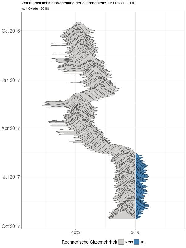
We visualize the posterior via "ridgeline plots" (formerly Joy plots)
Uses ggplot, ggridges, gganimate
(click here for animated version; also featured at Spektrum.de)

21 / 42

Joy/Ridges-Plot (Implementation)

gg_distrb <- ggplot(schw_gelb, aes(x = percent, y = date2,
    group=date2, frame=date, cumulative=TRUE, fill=..x..>50)) +
    geom_density_ridges_gradient(scale = 10, size = 0.25) +
    geom_vline(xintercept = 50, lty=1, lwd=1.2, col="grey90") +
    scale_fill_manual(
        name   = "Rechnerische Sitzemehrheit",
        breaks = c("FALSE", "TRUE"),
        labels = c("Nein", "Ja"),
        values = c("#d1d0ce", "steelblue") ) +
    theme(legend.position = "bottom")  +
    scale_x_continuous(labels = function(x) paste0(x, "%")) +
    scale_y_continuous(trans = rev_date) +
    guides(fill=guide_legend(override.aes=list(alpha=1))) +
    theme(
        axis.text    = element_text(size = rel(1.3)),
        axis.title.y = element_blank(),
        axis.title.x = element_blank(),
        legend.text  = element_text(size = rel(1.2)),
        legend.title = element_text(size = rel(1.3))) +
    labs(
        title = "Wahrscheinlichkeitsverteilung der Stimmanteile für Union - FDP",
        subtitle = "(seit Oktober 2016)")

22 / 42

Joy/Ridges-Plot (Implementation)

gg_distrb <- ggplot(schw_gelb, aes(x = percent, y = date,
    group=date, frame=date, cumulative=TRUE, fill=..x..>50)) +
   geom_density_ridges_gradient(scale = 10, size = 0.25) +
    # geom_vline(xintercept = 50, lty=1, lwd=1.2, col="grey90") +
    # scale_fill_manual(
    #     name   = "Rechnerische Sitzemehrheit",
    #     breaks = c("FALSE", "TRUE"),
    #     labels = c("Nein", "Ja"),
    #     values = c("#d1d0ce", "steelblue") ) +
    # theme(legend.position = "bottom")  +
    # scale_x_continuous(labels = function(x) paste0(x, "%")) +
    # scale_y_continuous(trans = rev_date) +
    # guides(fill=guide_legend(override.aes=list(alpha=1))) +
    # theme(
    #     axis.text    = element_text(size = rel(1.3)),
    #     axis.title.y = element_blank(),
    #     axis.title.x = element_blank(),
    #     legend.text  = element_text(size = rel(1.2)),
    #     legend.title = element_text(size = rel(1.3))) +
    # labs(
    #     title = "Wahrscheinlichkeitsverteilung der Stimmanteile für Union - FDP",
    #     subtitle = "(seit Oktober 2016)")

23 / 42

Animation

If you're able to ggplot, you are able to gganimate!
The gganimate package currently not on CRAN, install via:

devtools::install_github("drgtwo/gganimate")

library(ggplot2)
library(ggridges)
library(gganimate)
gg_distrb <- ggplot(schw_gelb, aes(x = percent, y = date,
         group=date, frame=date, cumulative=TRUE, fill=..x..>50)) +
    geom_density_ridges_gradient(scale = 10, size = 0.25)
gganimate(gg_distrb, "output.gif", interval=.2, ani.width=600)

Set GIF parameters (width, height, etc. via ani.options)
Control speed of the animation via interval argument
(lower values $\to$ higher speed)
Don't forget to set the frame argument in the call to ggplot (this is the variable over which the animation will iterate)
By setting cumulative=TRUE current frame also contains previous frames
Note: alpha argument does not work with *_gradient geoms

24 / 42

Frontend implementation

1) Creating a homepage with Shiny

2) Setting up the server with Shiny Server

3) APIs and stuff: tweetR and googlesheets

4) Keep the website running

25 / 42

26 / 42

Frontend - Shiny

Shiny in a nutshell:

R package by RStudio
Web application framework
Creation of interactive dashboards, running R in the background
Resources: Applied R Shiny Meetup, shiny.rstudio.com
Tip: Use shinydashboard for a more appealing dashboard UI

27 / 42

Frontend - Shiny

Shiny in a nutshell:

R package by RStudio
Web application framework
Creation of interactive dashboards, running R in the background
Resources: Applied R Shiny Meetup, shiny.rstudio.com
Tip: Use shinydashboard for a more appealing dashboard UI

Why Shiny?

Easy integration of interactive R output and calculations
No need for learning another language, Shiny creates the HTML, CSS and JavaScript for you!

27 / 42

Frontend - Shiny

28 / 42

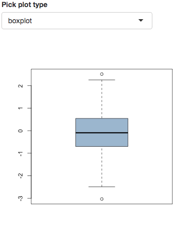
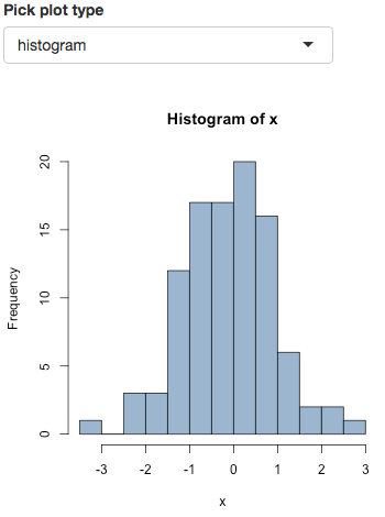
Frontend - Shiny

library(shiny)
ui <- fluidPage(
  selectInput("plotType_picker", "Pick plot type",
              choices = c("boxplot","histogram")),
  plotOutput("my_plot")
)
server <- function(input, output) {
  x <- rnorm(100)
  output$my_plot <- renderPlot({
    if (input$plotType_picker == "boxplot") {
      boxplot(x)
    } else
      hist(x)
  })
}
shinyApp(ui = ui, server = server)

29 / 42

Frontend - Shiny Server

Shiny Server in a nutshell:

Linux-based open source web server by RStudio
Access to the homepage starts an R process with a Shiny app on the server

Resources:

Official homepage

30 / 42

Frontend - Shiny Server

Setting up Shiny Server (on 64-bit Ubuntu 12.04+): (administrator's guide)

1) Install R and all needed R packages on the server

2) Install Shiny Server (install guide)

$ sudo apt-get install gdebi-core
$ sudo wget https://download3.rstudio.org/ubuntu-12.04/x86_64/shiny-server-1.5.3.838-amd64.deb
$ sudo gdebi shiny-server-1.5.3.838-amd64.deb

3) Customize the shiny-server.conf file to your needs

Tip 1:
'sanitize_errors false;'
gets you clearer error messages

Tip 2:

'app_idle_timeout 0;'

saves startup time of the R process

4) Put the Shiny files inside the path specified in shiny.server.conf

31 / 42

Frontend - Shiny Server

Capabilities of the free version (Shiny Server Open Source):

For non-commercial projects
Up to 20 users simultaneously
No multiple R processes!
→ code efficiently and precalculate results where possible

32 / 42

Frontend - Shiny Server

Capabilities of the free version (Shiny Server Open Source):

For non-commercial projects
Up to 20 users simultaneously
No multiple R processes!
→ code efficiently and precalculate results where possible

(R-based) alternatives:

Shiny Server Pro: Commercial use, multiple R processes etc.
shinyapps.io:
- Deploy Shiny apps on RStudio servers
- Free version limited to 25 hours of use per month!

32 / 42

Frontend - tweetR

The tweetR package in a nutshell:

Our use case: Send tweets with new results
Resources: user vignette, tweetR on GitHub
Alternative (more modern) package: rtweet

33 / 42

Frontend - tweetR

Sending a Tweet with tweetR:

1) Register a new Twitter app on apps.twitter.com

2) Use the credentials to do the authorization with R

setup_twitter_oauth(consumer_key = "your_consumer_key",
                    consumer_secret = "your_consumer_secret",
                    access_token = "your_access_token",
                    access_secret = "your_access_secret")

3) Start tweeting!

tweet(message = "Tweet tweet", mediaPath = "my_picture.png")

34 / 42

Frontend - googlesheets

The googlesheets package in a nutshell:

Our use case: Offering an API for our results
Resources: googlesheets on GitHub

35 / 42

Frontend - googlesheets

Exporting a table to Google Sheets with googlesheets:

1) Extract your credentials:

auth_info <- gs_auth()
saveRDS(auth_info, file = "auth_info.rds")

2) Use the credentials to do the authorization with R

gs_auth(token = "auth_info.rds")

3) Start uploading!

my_table <- data.frame("person"      = c("Sepp","Uli","Franz"),
                       "likes_koala" = c("yes", "yes", "yes"))
write.csv(my_table, file = "my_table.csv")
gs_upload("my_table.csv", sheet_title = "my_googleSheet",
          overwrite = TRUE)

36 / 42

Frontend - Keep the website running

Automation of the server:

We check hourly if new surveys are available and update the results
Implementation: see next slide
Tip: Automatic error notification using Pushbullet
- Supports notifications to all major (Desktop and mobile) systems
- R package: RPushbullet on GitHub

37 / 42

Implementation of the automation process

1) Set up the R script

while (1 < 2) { # do something eternally
  # Step 1: check for new surveys and perform calculations
  update_results()
  # Step 2: Update services with new results
  if (new_results) { # if new results are available
    send_tweet()
    export_googleSheets()
    # restart the server to fetch the new results (on Ubuntu 15.04+)
    system("sudo systemctl restart shiny-server")
  }
  # Step 3: Rest for an hour
  Sys.sleep(60*10)
}

2) Start the R script on the server

R CMD BATCH update_results_everyHour.R &

38 / 42

Outlook & sources

1) Future plans

2) Sources

39 / 42

Outlook - Future plans

Make frontend R package (shiny app) open source
Simplify data handling, Create online data base (with API), etc.
Extend the framework to:
- other elections (regional and international)
- improve interactive experience
- make @tagesschau (and others) use our methods!

40 / 42

Sources

General sources:

Raw voting intention polls: www.wahlrecht.de
Our slides are powered by Xaringan
tidyverse (previously hadleyverse)

41 / 42

Sources

General sources:

Raw voting intention polls: www.wahlrecht.de
Our slides are powered by Xaringan
tidyverse (previously hadleyverse)

How to reach us?

Visit us on koala.stat.uni-muenchen.de

Contact us directly: koala@stat.uni-muenchen.de
Feel free to contribute on GitHub

41 / 42

Preparing for election day

Keep in mind:

We do not make predictions!
Many voters (~40%) still undecided

42 / 42

Preparing for election day

Keep in mind:

We do not make predictions!
Many voters (~40%) still undecided

So, stay tuned...

... and follow us on Twitter :-)

42 / 42

Help

Keyboard shortcuts

↑, ←, Pg Up, k

Go to previous slide

↓, →, Pg Dn, Space, j

Go to next slide

Home

Go to first slide

End

Go to last slide

Number + Return

Go to specific slide

b / m / f

Toggle blackout / mirrored / fullscreen mode

Clone slideshow

Toggle presenter mode

Restart the presentation timer

?, h

Toggle this help