The framework is general in the sense that

(source: Bender, et al. (2020))

Consider setting with right-censored data:

• we observe (t_i, \delta_i), i = 1,\ldots, n, where
  • t_i = \min(T_i, C_i); T_i \sim F \perp C_i \sim G; T_i,C_i > 0
  • \delta_i = I(T_i \leq C_i) \in \{0,1\}

To approximate \lambda(t; \bfx_i) = \exp(g(\bfx_i(t), t)) \stackrel{PH}{=}\lambda_0(t)\exp(\bfx_i'\bsbeta)

• split the follow-up in J intervals (\kappa_{j-1}, \kappa_j], j = 1,\ldots, J

• assume piece-wise constant hazards: \begin{align} \lambda(t| \bfx_i(t)) & \equiv \exp(g(\bfx_{ij}, t_j)):=\lambda_{ij},\ \ \forall t \in (\kappa_{j-1}, \kappa_j],\\ \end{align}

• Estimation using
  • Piece-wise Exponential Model (PEM; e.g.: Laird, et al. (1981); Friedman (1982); Carstensen, et al. (2011))
  • Piece-wise exponential Additive Mixed Models (PAMM, e.g.: Cai, et al. (2002); Kauermann (2005); Argyropoulos, et al. (2015); Bender, et al. (2018))

\ra transform to PED using \kappa_0=0, \kappa_1 = 1, \kappa_2=1.5, \kappa_3=3

• define: \delta_{ij} = \begin{cases}1 & t_i \in (\kappa_{j-1}, \kappa_j] \wedge \delta_i = 1\\0 & \text{else}\end{cases}, t_{ij} = \begin{cases}t_{i}-\kappa_{j-1} & \delta_{ij}=1\\ \kappa_{j}-\kappa_{j-1}& \text{else}\end{cases}, t_j := \kappa_j

Competing risks setting with event types k \in \{1,2\}

\ra transform to PED using \kappa_0=0, \kappa_1 = 1, \kappa_2=1.5, \kappa_3=3

\ra estimate \lambda(t|\bfx, k) = \exp(f(\bfx(t_j),t_j,k)),\ \forall t\in(\kappa_{j-1}, \kappa_j],\ \ k \in \{1,2\}

PEM/GLM: \lambda(t) = \lambda_{0j} = \exp(\beta_{0j}), \forall t\in (\kappa_{j-1}, \kappa_j], j = 1,\ldots,J

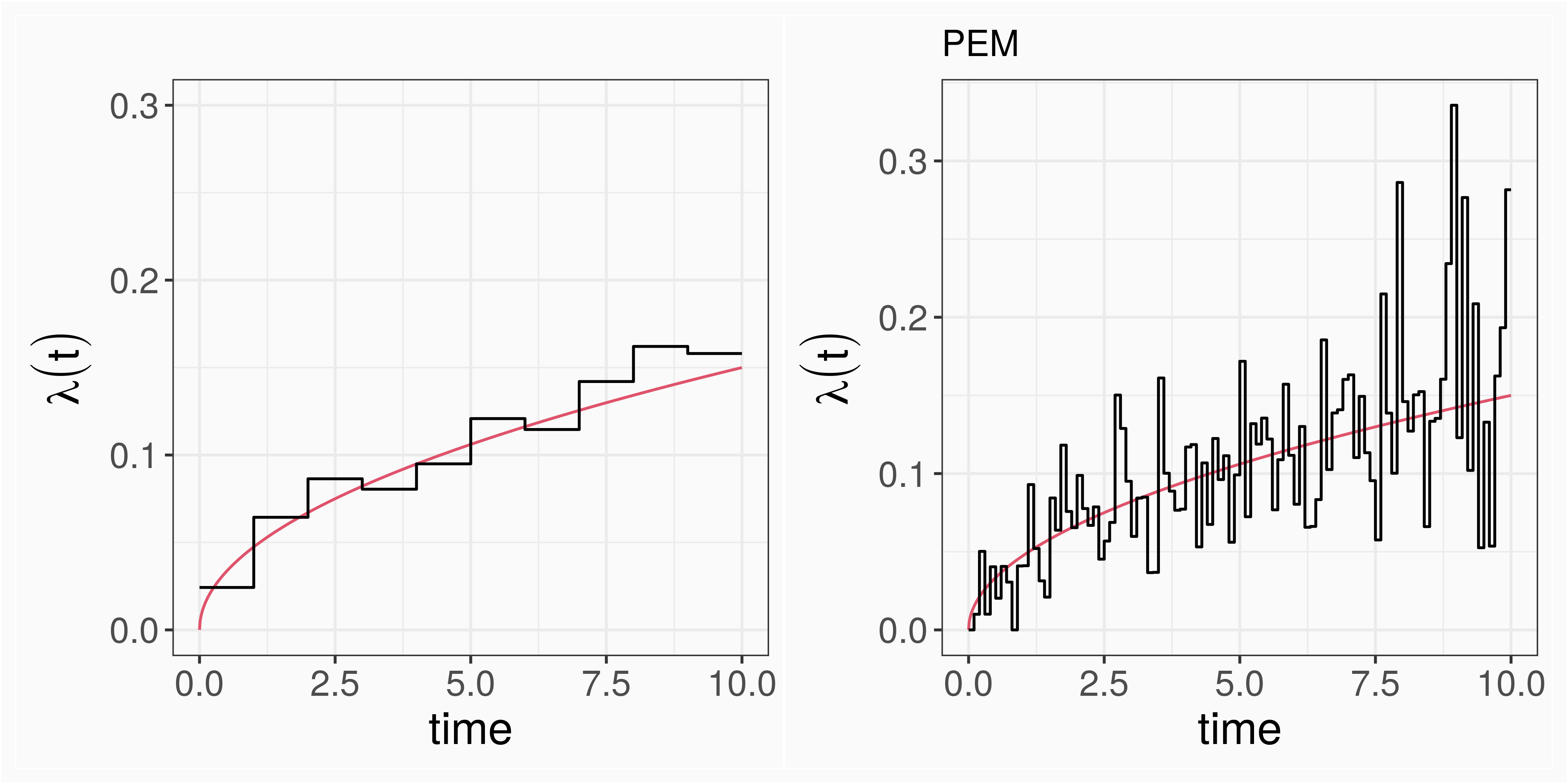
• trade of w.r.t. to number of split points (less flexible/more robust vs. more flexible/less robust)

• computationally inefficient (one parameter for each interval), especially when considering time-varying effects

• results sensitive to number and placement of interval cut points

PAMM/GAMM: \lambda(t) = \lambda_{0j} = \exp(f_0(t_j)), \forall t\in (\kappa_{j-1}, \kappa_j], j = 1,\ldots,J;\ f_0(t_j) = \sum_{q=1}^{Q}\beta_{0q}B_{0q}(t_j)

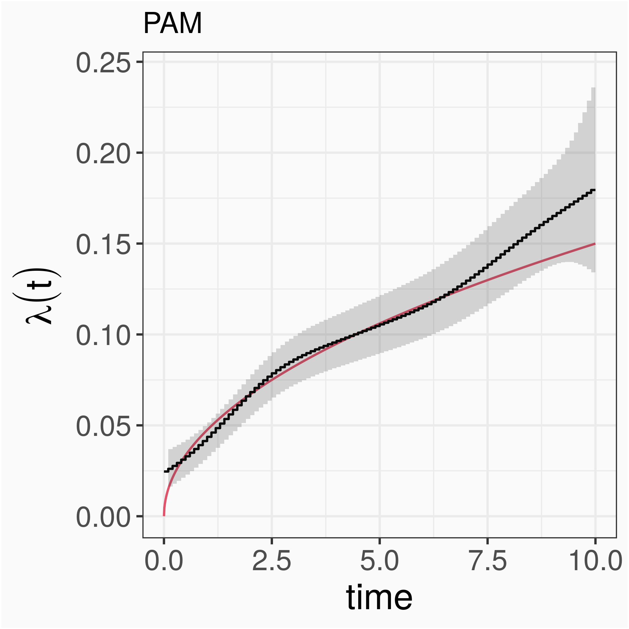
• large differences between neighboring coefficients/baseline hazards of neighboring intervals are penalized

• insensitive to number and placement of split points

• number of parameters to estimate determined by basis dimension Q, not number of intervals J

Time-varying effects

In the PEM/PAMM framework, time-varying effects are simply interactions of time t_j and other covariates.
\log(\lambda(t|x)) = f_{01}(t_j)I(complications = yes) + f_{02}(t_j)I(complications = no)

pam_tumor <- mgcv::gam(formula=ped_status~s(tend, by=complications), data=ped_tumor, family=poisson(), offset=offset)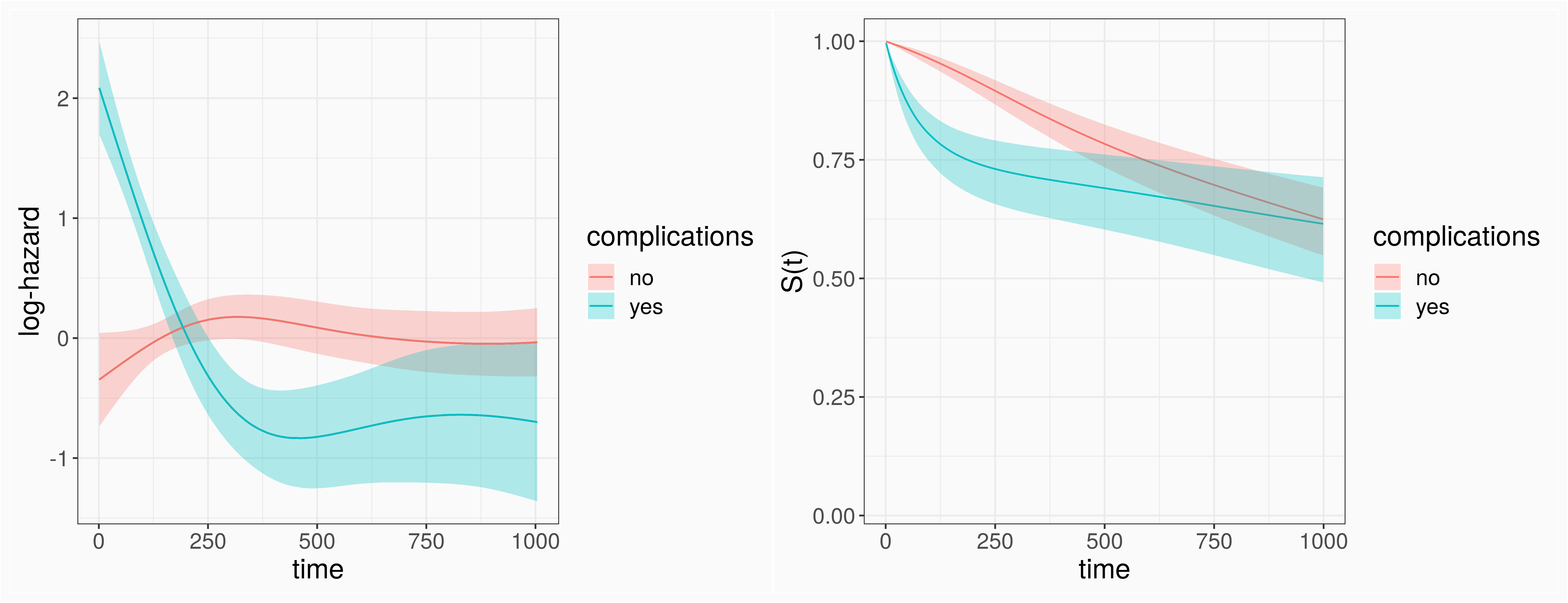

# "Regular" GAM
mgcv::gam(formula=ped_status~s(tend, by=complications), data=ped_tumor, family=poisson(), offset=offset)
# GAM with monotinicity constraints
scam::scam(formula=ped_status~s(tend, by=complications, bs = "mpd"), data=ped_tumor, family=poisson(), offset=offset)
# Bayesian GAM
brms::brm(formula=ped_status~s(tend, by=complications) + offset(offset), data=ped_tumor, family=poisson())

Competing Risks

\log(\lambda(t|x)) = f_{01}(t_j)I(k = 1) + f_{01}(t_j)I(k = 2) Cause specific hazards are time-varying effects of time t_j and covariate "event type" k

pam_cr <- mgcv::gam(formula = ped_status ~ s(tend, by = cause), data = ped_stacked, family = poisson(), offset = offset)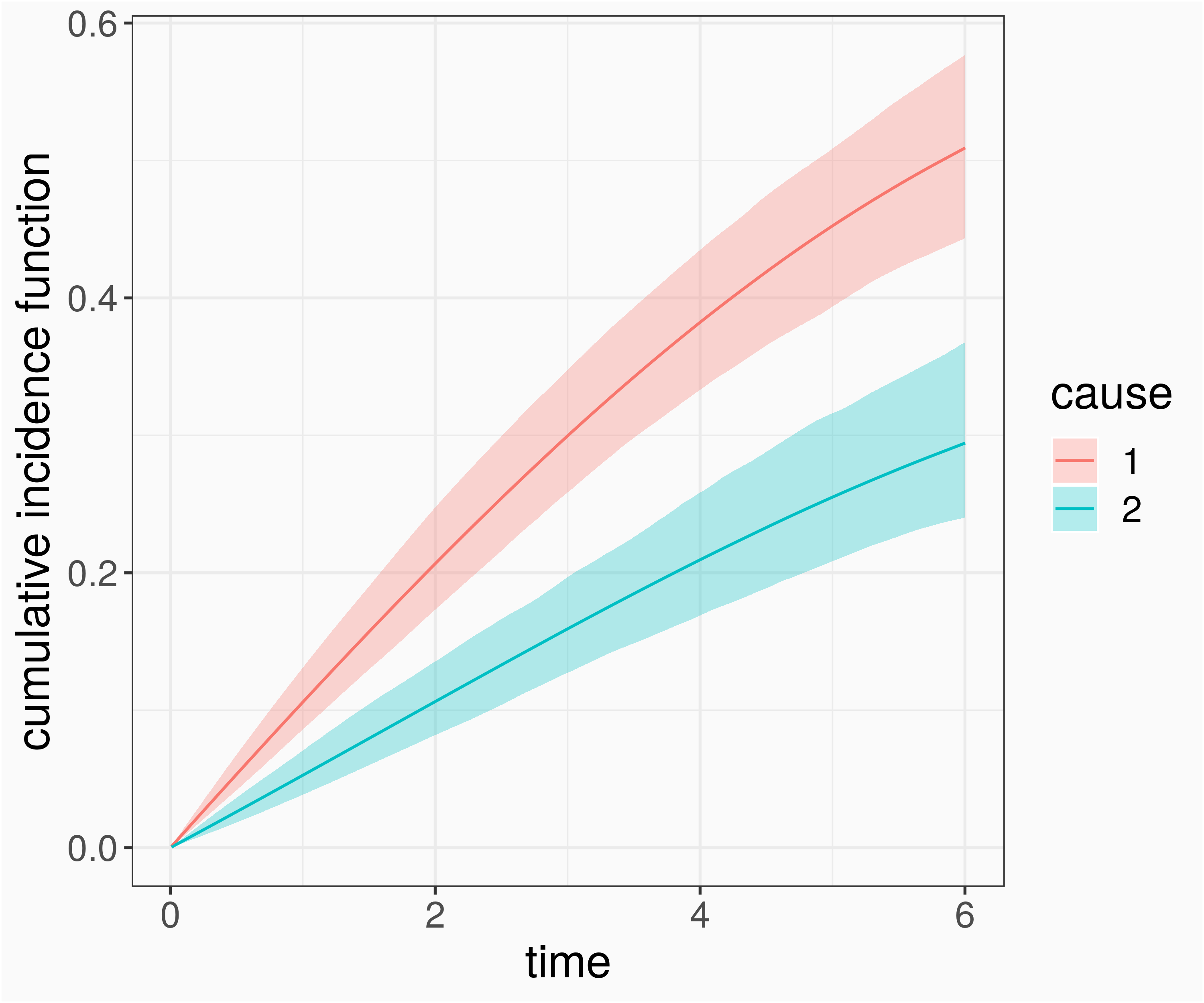

Tree based methods

Time-varying effects Shared vs. cause-specific effects (in CR)

(source: Bender, et al. (2020))

Outlook

• support for multi-state models

• facilitate extensions: S3 functions for calculation of hazard for other packages (e.g. mbooost, brms)

• Prototype for PEMs using xgboost available: https://github.com/adibender/pem.xgb

• However, ML algorithms need a different infrastructure (resampling, tuning, benchmarking)
  \ra Development will probably continue in mlr3 and mlr3proba (Lang, et al. (2019); Sonabend, et al. (2020))

References

Argyropoulos, C. et al. (2015). "Analysis of Time to Event Outcomes in Randomized Controlled Trials by Generalized Additive Models". In: PLoS ONE 10.4, p. e0123784. DOI: 10.1371/journal.pone.0123784. URL: http://dx.doi.org/10.1371/journal.pone.0123784.

Bender, A. et al. (2018). "A generalized additive model approach to time-to-event analysis". En. In: Statistical Modelling 18.3-4, pp. 299-321. ISSN: 1471-082X. DOI: 10.1177/1471082X17748083.

Bender, A. et al. (2020). "A General Machine Learning Framework for Survival Analysis". In: arXiv:2006.15442 [cs, stat]. arXiv: 2006.15442.

Cai, T. et al. (2002). "Mixed Model-Based Hazard Estimation". In: Journal of Computational and Graphical Statistics 11.4, pp. 784-798. ISSN: 1061-8600. DOI: 10.1198/106186002862. URL: http://dx.doi.org/10.1198/106186002862.

Carstensen, B. et al. (2011). "Using Lexis Objects for Multi-State Models in R". En. In: Journal of Statistical Software 38.1. Number: 1, pp. 1-18. ISSN: 1548-7660. DOI: 10.18637/jss.v038.i06. URL: https://www.jstatsoft.org/index.php/jss/article/view/v038i06.

Friedman, M. (1982). "Piecewise Exponential Models for Survival Data with Covariates". In: The Annals of Statistics 10.1, pp. 101-113. ISSN: 00905364. URL: http://www.jstor.org/stable/2240502.

References

Kauermann, G. (2005). "Penalized spline smoothing in multivariable survival models with varying coefficients". In: Computational Statistics & Data Analysis 49.1, pp. 169-186. ISSN: 0167-9473. DOI: 10.1016/j.csda.2004.05.006. URL: http://www.sciencedirect.com/science/article/pii/S0167947304001240.

Laird, N. et al. (1981). "Covariance Analysis of Censored Survival Data Using Log-Linear Analysis Techniques". In: Journal of the American Statistical Association 76.374, pp. 231-240. DOI: 10.2307/2287816. URL: http://www.jstor.org/stable/2287816.

Lang, M. et al. (2019). "mlr3: A modern object-oriented machine learning framework in R". In: Journal of Open Source Software. DOI: 10.21105/joss.01903. URL: https://joss.theoj.org/papers/10.21105/joss.01903.

Sonabend, R. et al. (2020). "mlr3proba: Machine Learning Survival Analysis in R". In: arXiv:2008.08080 [cs, stat]. arXiv: 2008.08080. URL: http://arxiv.org/abs/2008.08080 (visited on Aug. 20, 2020).