Penalized Estimation of Cumulative Effects
Andreas Bender, F Scheipl, W Hartl, A G Day, H Küchenhoff
Departement of Statistics, LMU Munich
2017/12/17
Outline
Motivation
Exposure-Lag-Response Associations
Application
Motivation
Multi-center study of critical care patients from 457 ICUs (
≈10kpatients)maximum follow up of 60 days (we only consider short term survival
t≤30)Various confounders:
- Age, Gender, BMI
- Diagnosis, Admission Category
- year of ICU admission
- Apache II Score
- ICU random effect
11-day nutrition protocol
- prescribed calories (determined at baseline
t=0) - daily caloric intake
- daily caloric adequacy (CA) = caloric intake/prescribed calories
- prescribed calories (determined at baseline
Caloric Intake
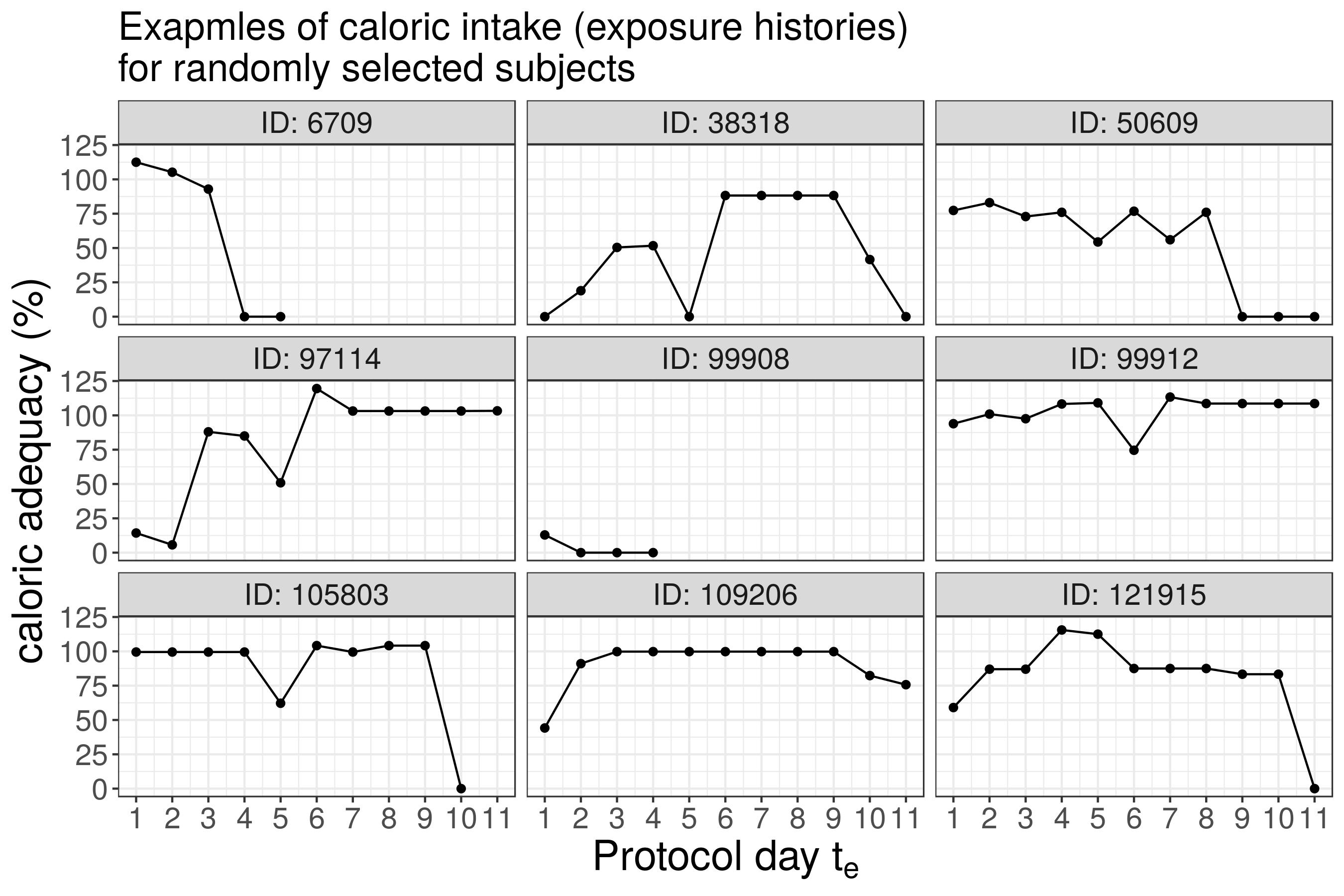
Motivation
We are interested in how artificial nutrition (exposure) affects short term survival (outcome)
Difficulty:
effect of nutrition might have a temporal delay (e.g. nutrition today affects survival 4 days later)
effect of nutrition might "wear off" after some time (e.g. nutrition on day 1 likely won't affect the hazard on day 30)
the (delayed) effect of nutrition also depends on the amount of nutrition (caloric adequacy) provided, possibly non-linearly
the same amount of exposure might have a different effect depending on the follow up and exposure time
the effect may be cumulative (i.e., 5 days of malnutrition in a row may be worse than only 2 in a row or 5 days malnutrition scattered throughout the follow up while on the other days "correct" amount was provided)
Terminology
We use the following terminology and notation:
Time-to-event
t: Time at which event times are observedTime of exposure
te: Time at which values of the exposure are observed (must not necessarily overlap temporally witht, measured in the same units or be in the same domain ast, e.g. calendar days (te) vs. 24h periods (days) since admission to ICUt)time-varying effects (TVE): Effects of time-constant covariates (covariates observed at the beginning of the follow-up) that can vary over time
ttime-dependent covariates (TDC): Covariates whose values change over time. Value changes are recorded at exposure time
te(here synonymous to exposure)Exposure value
z(te): The value of the TDC observed at exposure timeteExposure history
z: The complete history of observed values of the exposure/TDCz=(z(te,1),z(te,2),...,z(te,Q))
Terminology
A general cumulative effect/Exposure-Lag-Response Association (ELRA) can be defined as
g(z,t)=∫te:te≤th(t,te,z(te))dte
Partial effects
h(t,te,z(te)): The effect of the TDC recorded at exposure timetewith valuez(te)on the hazard at follow up timet(the tri-variate functionhis potentially non-linear in all three dimensions)Cumulative effect
g(z,t): The total (cumulated) effect of the partial effects on the log-hazard at timetgiven exposure historyz
Lag-Lead-Window
The integration borders can be defined more general, such that
g(z,t)=∫t−tlagt−tlag−tleadh(t,te,z(te))dte
- Lag time
tlag: The length of the delay until the TDC recorded at exposure timetestarts to affect the hazard (oftentlag=0) - Lead time
tlead: The duration of the effect of the TDC observed at exposure timete tlagandtleaddefine the set of exposures that contribute to the cumulative effect at timetas{z(te):te∈[t−tlag−tlead,t−tlag]}- Minimal requirement:
∫te:te≤t - Special case
∫t0follows withtlag=0andtlead=t - Example (
tlag=4,tlead=3):- The last nutrition that will enter the cumulative effect at
time
t=10is nutrition atte≤t−tlag=10−4=6, i.e.z(te=6) - The earliest nutrition that will contribute to the cumulative effect at time
t=10is nutrition atte≥t−tlag−tlead=10−4−3=3
- The last nutrition that will enter the cumulative effect at
time
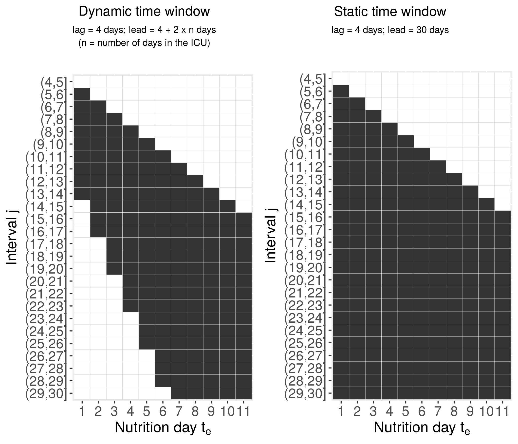
Lag-Lead-Window
The integration borders can be defined even more general, such that
g(z,t)=∫t−tlag(te)t−tlag(te)−tlead(te)h(t,te,z(te))dte=∫Te(t)h(t,te,z(te))dte
tlagandtleadtimes can themselves depend on (exposure) timeTe(t)is the set of exposure timesterelevant to the cumulative effect at timetWe call
Te(t)the Lag-Lead-Window or Window of effectiveness
Lag-Lead Window (Example)
ELRAs in the literature
Some models known from the literature follow as special cases of the general
specification
g(z,t)=∫Te(t)h(t,te,z(te))
when we assume that partial effects h only depend on latency t−te
instead of concrete combination of t and te, i.e.,
h(t=30,te=3,z(te))!=h(t=40,te=13,z(te))!=~h(t−te=27,z(te))
WCE: Weighted Cumulative Exposure (Sylvestre and Abrahamowicz, 2009):
g(z,t)=∫Te(t)h(t−te)z(te)Also possible within general framework:
- more flexible WCE:
g(z,t)=∫Te(t)h(t,te)z(te) - time-varying DLNM (TV DLNM):
g(z,t)=∫Te(t)h(t,t−te,z(te))
- more flexible WCE:
Exposure-Lag-Response Association
g(z,t)represents the cumulative, time-varying effect of exposure historyzon the log-hazard at timetwe define its contribution to the model's additive predictor as
g(zi,t)=∫Te(t)h(~tj,te,zi(te))dte≈∑q:te,q∈Te(t)Δqh(~tj,te,q,zi(te,q))∀t∈(κj−1,κj],
with
~tj:=(κj−κj−1)/2,j=1,…,J- partial effects
h(~tj,te,zi(te)) - quadrature weights
Δq=te,q−te,q−1for numerical integration are given by the time between two consecutive exposure measurements
Tensor product smooths
Low rank representation of the tri-variate smooth function
h(t,te,z(te))=L∑ℓ=1R∑r=1M∑m=1γℓrmBm(z(te))Br(te)Bℓ(t)
with
model matrix
X=Xt⊙Xte⊙Xz(te)andpenalty
S=νz(te)IdR⊗IdL⊗Sz(te)+νteIdL⊗Ste⊗IdM+νtSt⊗IdR⊗IdM
→ Estimate parameters γ by optimizing
D(γ)+∑kνkγ′Skγ (Wood, 2011), where
D(γ)is the model deviance (of the Poisson GAMM)γcontains all Spline basis coefficients and random effectsνkandSk,k=1,…,Kare the smoothing parameters and penalty matrices for thek-th smooth term, respectively
Exposure-Lag Response Association
- If we restrict the ELRA to be linear in the exposure, i.e.,
h(zi(te),te,t)=~h(te,t)⋅zi(te)we can simplify tog(zi,t)≈Q∑q=1~Δi,q~h(te,q,t)with~Δi,q={zi(te,q)Δq if te,q∈Te(t)0 else
Exposure-Lag Response Association
Spline bases for the bivariate functions
~h(te,t)are set up via tensor product B-spline basis with marginal basesBm(te),m=1,…,MandBk(t),k=1,…,Kdefined over the exposure and hazard time domains, respectivelyMandKdelimit the maximal complexity of the ELRA~h(te,t)=∑Mm=1∑Kk=1γm,kBm(te)Bk(t)Combining above equations yields:
g(zi,t)≈M∑m=1K∑k=1γm,k~Bi,m(te,t)Bk(t),where~Bi,m(te,t)=∑Qq=1~Δi,qBm(te).
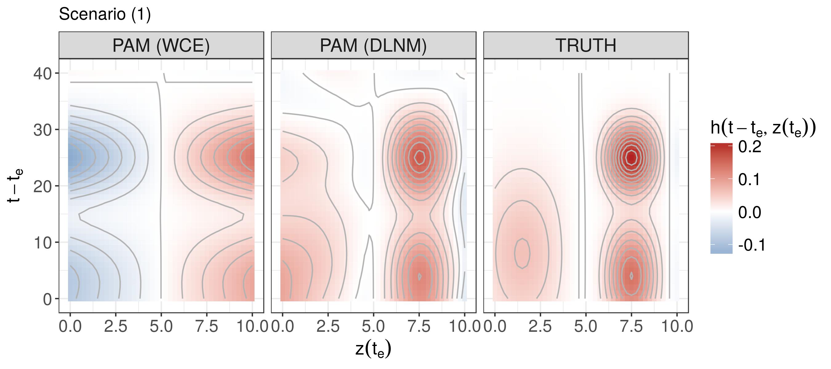
Simulation - DLNM
λ(t|z)=λ0(t)exp(∫h(t−te,z(te))dte)t∈(0,40],te∈[−40,40],z(te)∈[0,10]
Simulation (2) - TV DLNM
λ(t|z)=λ0(t)exp(∫~h(t,t−te,z(te))dte)=λ0(t)exp(∫f(t)⋅h(t−te,z(te))dte) and
f(t)=−cos(πt/tmax)
Application
In the application example (categorical nutrition), we estimate
log(λi(t|xi,zi,ℓi))=f0(t)+P∑p=1fp(xi,p,t)+g(zi,t)+bℓi
with
f0(tj)=∑Mm=1γ0mBm(tj)represents the log baseline-hazardf(xi,p,tj)=∑Mm=1∑Lℓ=1γmℓBm(xi,p)Bℓ(tj)are potentially non-linear, potentially non-linearly time-varying effects of confoundersxi,pg(zi,t)=gC2(zC2i,t)+gC3(zC3i,t)zC2iandzC3idummy variables that indicate whether subjectireceived categoryC2andC3nutrition on dayte,q,q=1,…,11, respectivelygC2(zi,t)≈∑Qq=1~ΔC2i,q~hC2(te,q,t)
bℓiis the random effect associated with ICU (cluster)ℓiat which subjectiis treated
→C1 reference category
PAMM
- We know how the estimate such models in the framework of
Generalized Additive Mixed Models (GAMMs)
Fortunately, we can fit survival models via Poisson GLMs/GAMMs by representing them as a Piece-wise exponential Additive Mixed Model (PAMMs)
to do so requires to
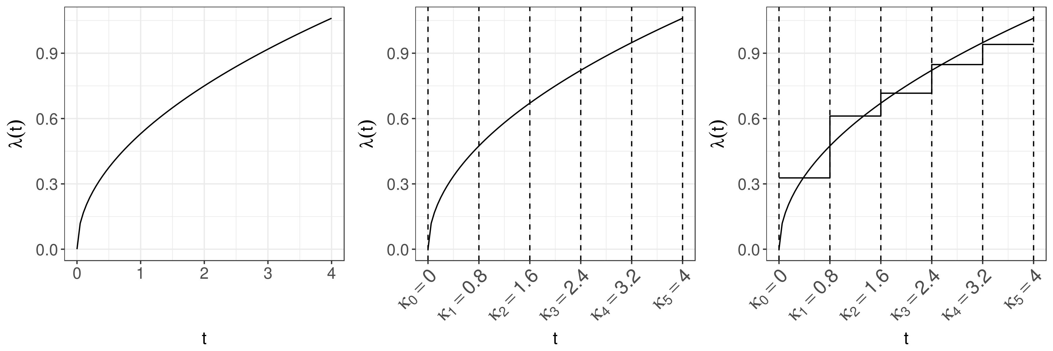
- divide the follow up
(0,tmax]intoJintervals withJ+1cut-points0=κ0<…<κJ=tmax - transform the data into appropriate format (pseudo observations in
each interval):
- interval specific event-indicators
δij, whereδij=1if subjectiexperienced an event in intervalj(i.e.ti∈(κj−1,κj]andTi<Ci) andδij=0else - offsets
oij=log(tij), wheretij=min(ti−κj−1,κj−κj−1)is the time subjectispent in intervalj
- interval specific event-indicators
- in the
jthinterval(κj−1,κj]estimate a piece-wise constant hazard rateλ(t)=λj ∀ t∈(κj−1,κj](more intervals lead to better approximation)
- divide the follow up
Application (Results)
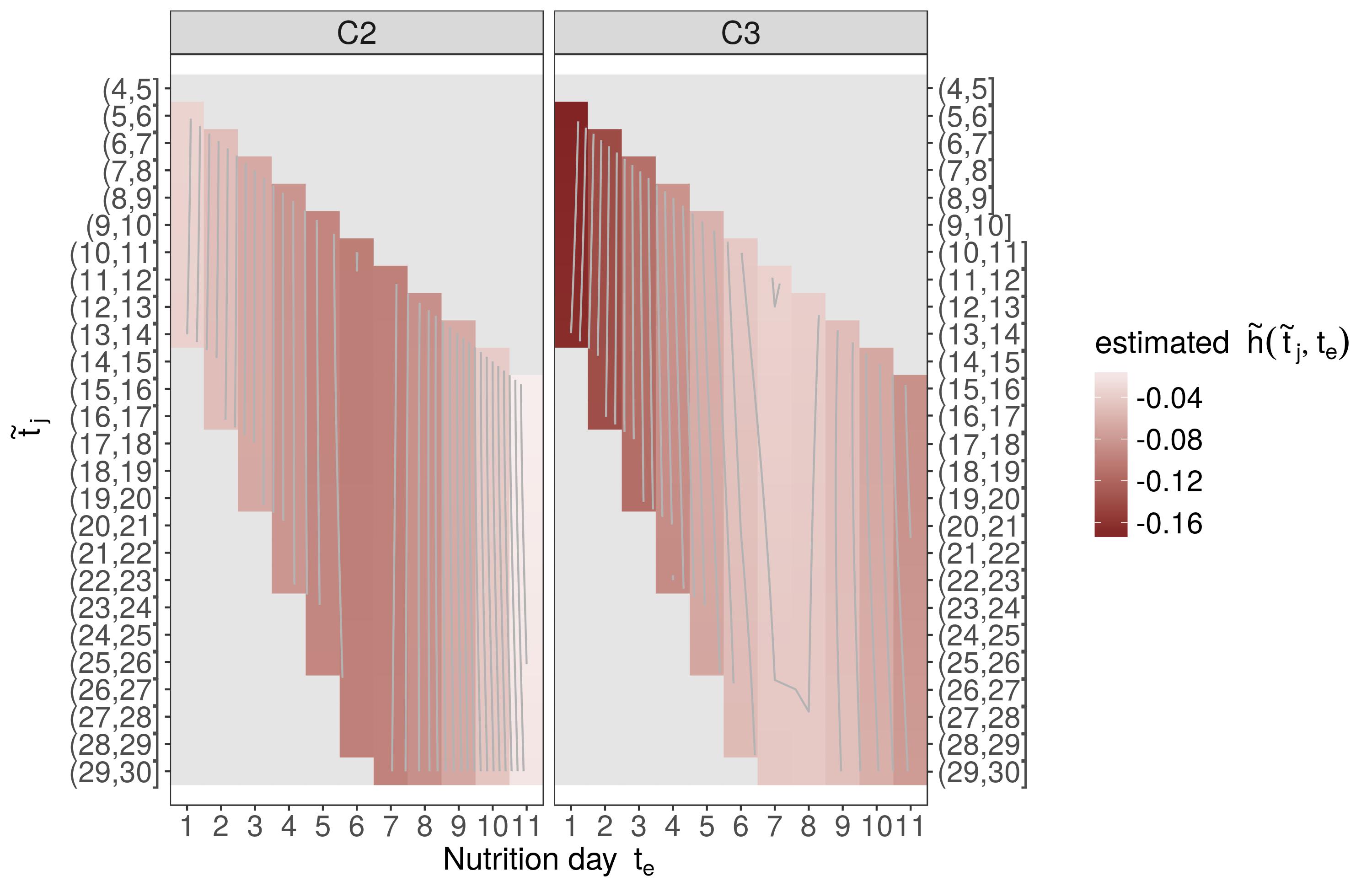
Application (Results)
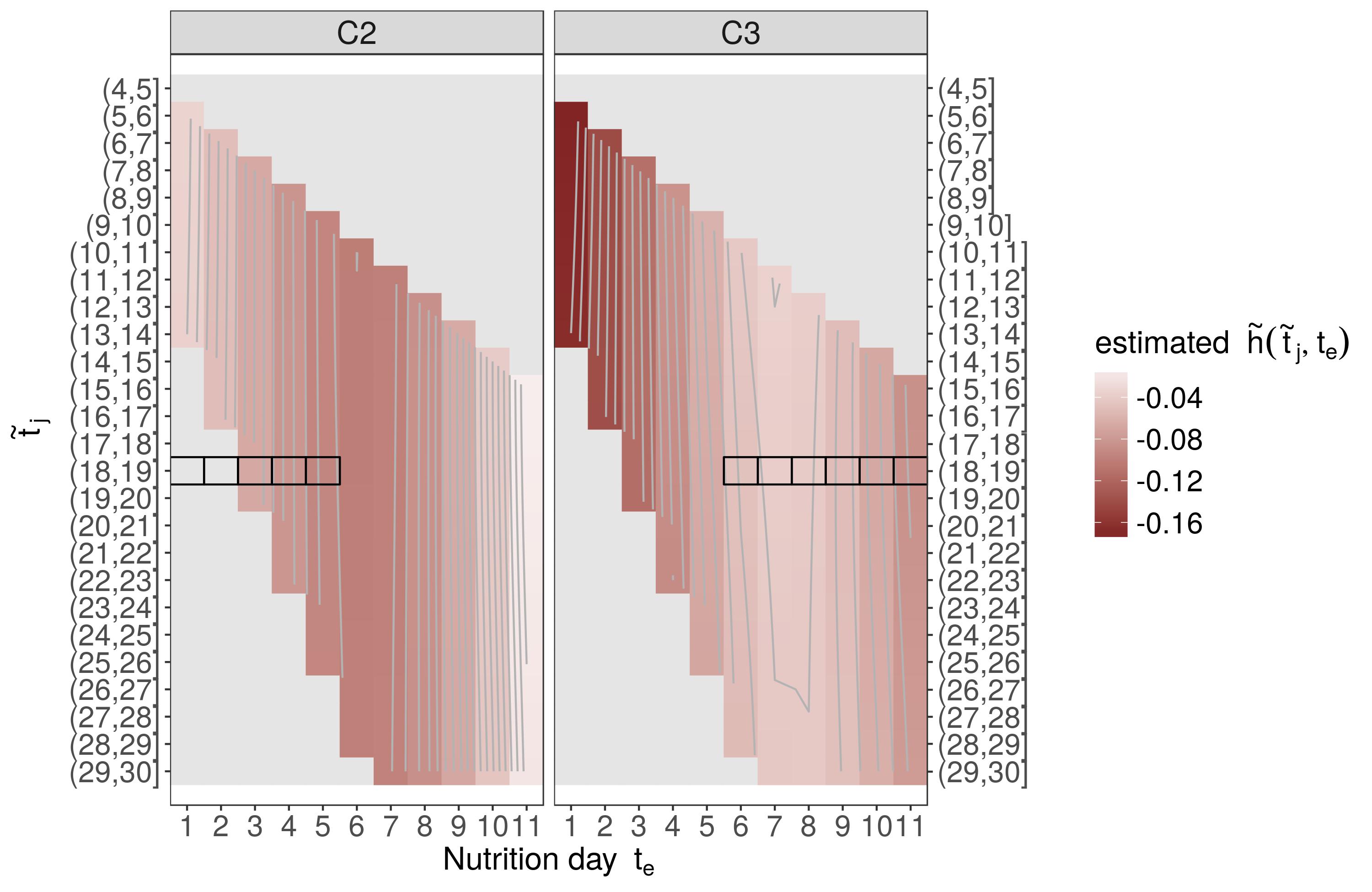
Example:
z=(5×C2,6×C3)zC2=(1,1,1,1,1,0,0,0,0,0,0),zC3=(0,0,0,0,0,1,1,1,1,1,1)g(z,~tj=18.5)=g(zC2,18.5)+g(zC3,18.5)≈−0.57
→ Risk reduction of exp(−0.57)=0.57 compared to subject with 11×C1 nutrition (c.p)
Application (Results)
These bivariate surfaces are difficult to interpret as
they must be interpreted with respect to a subject who received
C1nutrition on all 11 days of nutrition protocolpartial effects
hC2(t,te)andhC3(t,te)can both contribute to the cumulative effect, depending on the specific nutrition profilefor these reasons, we prefer to analyze and interpret estimated hazard ratios between hypothetical patients with different clinically relevant exposure histories (
z1andz2)
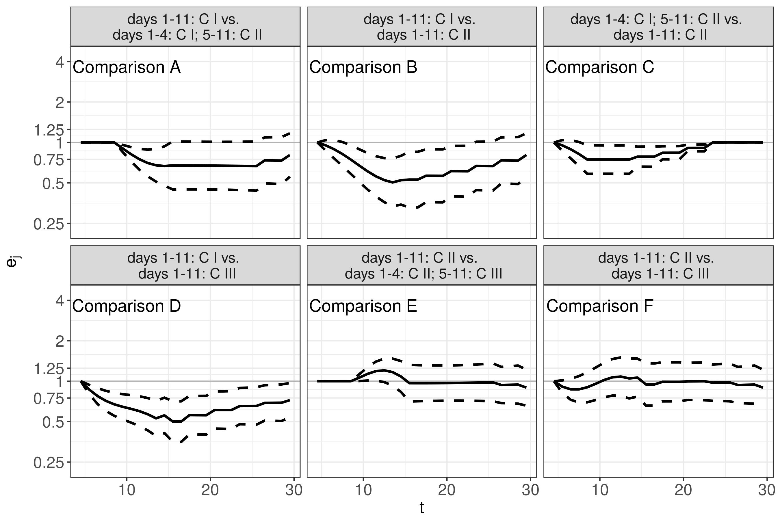
ej=λ(~tj|z2)λ(~tj|z1)
Application (Results)
We compare the following nutrition profiles:
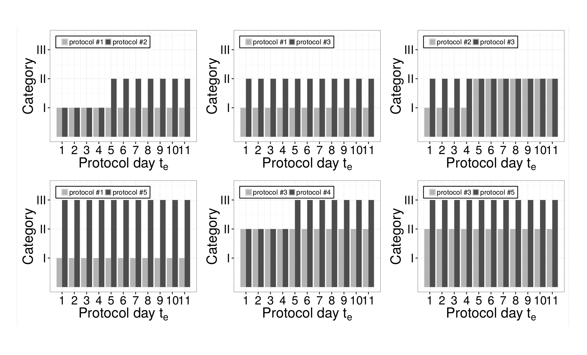
Application (Results)
→ Complete, mildly hypocaloric nutrition reduces risk of mortality
compared to a complete, severely hypocaloric nutrition (Comparison B)
→ No further risk reduction when moving from mildly hypocaloric to
partial or complete near target nutrition (Comparisons E, F)
→ Sensitivity analyses (Imputation of missing protocols,
lag/lead specification, penalty structure, ...) show no substantive deviation
from main results
Limitations (and outlook)
currently,
tlagandtleadmust be specified a priori→would be nice if the lag-lead window could be selected data-driven (e.g. Obermeier et al., 2015)we assume that patients released from hospital survived until the end of the follow-up (
t=30). Sensitivity analysis with hospital discharge as censoring event do not change the results→Competing risks model for outcomes hospital discharge and death would be preferableModeling and interpretation of TDCs always difficult, especially if exogeneity is unclear, e.g.
- although nutrition is provided by hospital staff, amount provided might depend on patients' health status
- more recent values provide better confounder adjustment but may also be fully indicative of the outcome (indication bias)
Model choice becomes difficult when all effects are potentially non-linear and/or non-linearly time-varying (boosting ad double-penalty procedures promising)
Links and Acknowledgments
- Talk is based on two publications
- Andreas Bender, Andreas Groll, and Fabian Scheipl. 2018. “A Generalized Additive Model Approach to Time-to-Event Analysis.” Statistical Modelling. https://doi.org/10.1177/1471082X17748083.
- Andreas Bender, Fabian Scheipl, Wolfgang Hartl, Andrew G Day, Helmut Küchenhoff; "Penalized estimation of complex, non-linear exposure-lag-response associations", Biostatistics, , kxy003, https://doi.org/10.1093/biostatistics/kxy003
pammtools: Package for Piece-wise exponential Additive Mixed Models (in development)

Slides created via Yihui Xie's R package xaringan with (modified) Metropolis theme
All graphics have been created using Hadley Whickham's ggplot2
Models are estimated using Simon Wood's mgcv

References
- Friedman, Michael. “Piecewise Exponential Models for Survival Data with Covariates.” The Annals of Statistics 10, no. 1 (1982): 101–113.
- Gasparrini, Antonio. “Modeling Exposure–lag–response Associations with Distributed Lag Non-Linear Models.” Statistics in Medicine 33, no. 5 (February 28, 2014): 881–99. https://doi.org/10.1002/sim.5963.
- Gasparrini, Antonio, Fabian Scheipl, Ben Armstrong, and Michael G. Kenward. “A Penalized Framework for Distributed Lag Non-Linear Models.” Biometrics, January 1, 2017. https://doi.org/10.1111/biom.12645.
- Holford, Theodore R. “The Analysis of Rates and of Survivorship Using Log-Linear Models.” Biometrics 36, no. 2 (1980): 299–305. https://doi.org/10.2307/2529982.
- Laird, Nan, and Donald Olivier. “Covariance Analysis of Censored Survival Data Using Log-Linear Analysis Techniques.” Journal of the American Statistical Association 76, no. 374 (1981): 231–240. https://doi.org/10.2307/2287816.
- Marra, Giampiero, and Simon N. Wood. “Coverage Properties of Confidence Intervals for Generalized Additive Model Components.” Scandinavian Journal of Statistics 39, no. 1 (March 1, 2012): 53–74. https://doi.org/10.1111/j.1467-9469.2011.00760.x.
- Sylvestre, Marie-Pierre, and Michal Abrahamowicz. “Flexible Modeling of the Cumulative Effects of Time-Dependent Exposures on the Hazard.” Statistics in Medicine 28, no. 27 (2009): 3437–3453. https://doi.org/10.1002/sim.3701.
References
- Whitehead, John. “Fitting Cox’s Regression Model to Survival Data Using GLIM.” Journal of the Royal Statistical Society. Series C (Applied Statistics) 29, no. 3 (1980): 268–75. https://doi.org/10.2307/2346901.
- Wood, Simon N. Generalized Additive Models: An Introduction with R. Boca Raton and FL: Chapman & Hall/CRC, 2006.
- Wood, Simon N. “Low-Rank Scale-Invariant Tensor Product Smooths for Generalized Additive Mixed Models.” Biometrics 62, no. 4 (December 1, 2006): 1025–36. https://doi.org/10.1111/j.1541-0420.2006.00574.x.
- Wood, Simon N. “Fast Stable Restricted Maximum Likelihood and Marginal Likelihood Estimation of Semiparametric Generalized Linear Models.” Journal of the Royal Statistical Society: Series B (Statistical Methodology) 73, no. 1 (2011): 3–36. https://doi.org/10.1111/j.1467-9868.2010.00749.x.
- Wood, Simon N. “On P-Values for Smooth Components of an Extended Generalized Additive Model.” Biometrika 100, no. 1 (March 1, 2013): 221–28. https://doi.org/10.1093/biomet/ass048.
- Wood, Simon N., Fabian Scheipl, and Julian J. Faraway. “Straightforward Intermediate Rank Tensor Product Smoothing in Mixed Models.” Statistics and Computing, 2012. https://doi.org/10.1007/s11222-012-9314-z.
References
- Wickham, Hadley. Ggplot2: Elegant Graphics for Data Analysis. 2nd ed. 2016. New York, NY: Springer, 2016.
- Yihui Xie (2017). xaringan: Presentation Ninja. R package version 0.4.4. https://github.com/yihui/xaringan
- Hadley Wickham, Romain Francois, Lionel Henry and Kirill Müller (2017). dplyr: A Grammar of Data Manipulation. R package version 0.7.4. https://CRAN.R-project.org/package=dplyr
Caloric Adequacy
caloric intake = calories from EN + PN + PF
caloric adequacy (CA):
CA(%)=caloric intake/prescribed calories⋅100discretized caloric adequacy (in 3 categories):
C1:0%≤CA<30%and no OIC2:30%≤CA<70%and no OI or0%≤CA<30%and additional OI
C3:CA≥70%or30%≤CA<70%and additional OI