pammtools
Survival Analysis with Generalized Additive Mixed Models
R Medicine 2020
Andreas Bender (@adibender),
Fabian Scheipl, Philipp Kopper
Department of Statistics, LMU Munich
Time-to-event Analysis (Survival Analysis) requires special methods because
outcome can not always be fully observed (censoring, truncation)
covariate values can change over time (time-varying covariates)
covariate effects can change over time (time-varying effects)
competing events prevent observation of the event of interest (competing risks)
observation units transition between different states (recurrent events, multi-state models)
\usepackageamsmath,amssymb,bm
Hitorically Survival Analysis dominated by Cox type models
Many Survival Models can be represented as Poisson Regression (on transformed data)
Piece-wise Exponential Model (PEM; estimation based on GLM)
e.g., Laird and Olivier (1981); Friedman (1982)Piece-wise exponential Additive Mixed Model (PAMM; estimation based on GAMM)
e.g., Cai, Hyndman, and Wand (2002); Bender, Groll, and Scheipl (2018)
→ Use any method/R package for Survival Analysis that supports optimization
of Poisson Likelihood (e.g., GAMMs via mgcv; Wood (2017))
\usepackageamsmath,amssymb,bm

\usepackageamsmath,amssymb,bm
Survival Analysis as Poisson Regression

→ transform to PED using intervals cut points 0,1,1.5 and 3

→ transform to PED using intervals cut points 0,1,1.5 and 3

→ transform to PED using intervals cut points 0,1,1.5 and 3

→ transform to PED using intervals cut points 0,1,1.5 and 3

→ transform to PED using intervals cut points 0,1,1.5 and 3

The pammtools package
pammtools facilitates
data transformation (
as_ped):- right-censoring
- competing risks
post-processing:
- prediction (
add_hazard,add_surv_prob,add_cif), - model evaluation (integrated brier score via
pec)
- prediction (
convenience functions
library(pammtools)data("tumor")| days | status | age | sex | complications |
|---|---|---|---|---|
| 311 | 1 | 65 | male | no |
| 469 | 0 | 82 | female | no |
| 1257 | 1 | 66 | female | no |
| 1 | 1 | 96 | female | yes |
| 13 | 1 | 72 | male | yes |
| 1542 | 0 | 29 | male | yes |
Data Transformation
ped <- tumor %>% as_ped(Surv(days, status) ~ .)| id | tstart | tend | interval | offset | ped_status | age | sex | complications |
|---|---|---|---|---|---|---|---|---|
| 167 | 0 | 1 | (0,1] | 0.0000000 | 0 | 64 | male | yes |
| 167 | 1 | 2 | (1,2] | 0.0000000 | 0 | 64 | male | yes |
| 167 | 2 | 3 | (2,3] | 0.0000000 | 0 | 64 | male | yes |
| 167 | 3 | 5 | (3,5] | 0.6931472 | 0 | 64 | male | yes |
| 167 | 5 | 6 | (5,6] | 0.0000000 | 0 | 64 | male | yes |
| 167 | 6 | 7 | (6,7] | 0.0000000 | 0 | 64 | male | yes |
| 167 | 7 | 8 | (7,8] | 0.0000000 | 1 | 64 | male | yes |
| 397 | 0 | 1 | (0,1] | 0.0000000 | 0 | 68 | female | yes |
| 397 | 1 | 2 | (1,2] | 0.0000000 | 0 | 68 | female | yes |
| 397 | 2 | 3 | (2,3] | 0.0000000 | 1 | 68 | female | yes |
Propportional Hazards Model
pam1 <- mgcv::gam( formula = ped_status ~ s(tend) + sex + complications + s(age), data = ped, family = poisson(), offset = offset)summary(pam1)## Parametric coefficients:## Estimate Std. Error z value Pr(>|z|)## (Intercept) -7.86165 0.08396 -93.632 < 2e-16 ***## sexfemale 0.12095 0.10604 1.141 0.254## complicationsyes 0.68619 0.10695 6.416 1.4e-10 ***## Approximate significance of smooth terms:## edf Ref.df Chi.sq p-value## s(tend) 3.794 4.717 19.83 0.00116 **## s(age) 4.903 5.920 28.56 8.04e-05 ***...Hazard
hazard_df <- ped %>% make_newdata(tend = unique(tend), complications = unique(complications)) %>% add_hazard(pam1) # age fixed at mean, sex at modus value| interval | tend | complications | hazard | ci_lower | ci_upper |
|---|---|---|---|---|---|
| (0,1] | 1 | no | 0.0005227 | 0.0003787 | 0.0007215 |
| (1,2] | 2 | no | 0.0005219 | 0.0003783 | 0.0007198 |
| (2,3] | 3 | no | 0.0005210 | 0.0003780 | 0.0007181 |
| (0,1] | 1 | yes | 0.0010381 | 0.0007420 | 0.0014524 |
| (1,2] | 2 | yes | 0.0010365 | 0.0007414 | 0.0014491 |
| (2,3] | 3 | yes | 0.0010348 | 0.0007407 | 0.0014458 |
Survival Porbability
surv_prob <- ped %>% make_newdata(tend = unique(tend), complications = unique(complications)) %>% group_by(complications) %>% # important !! add_surv_prob(pam1)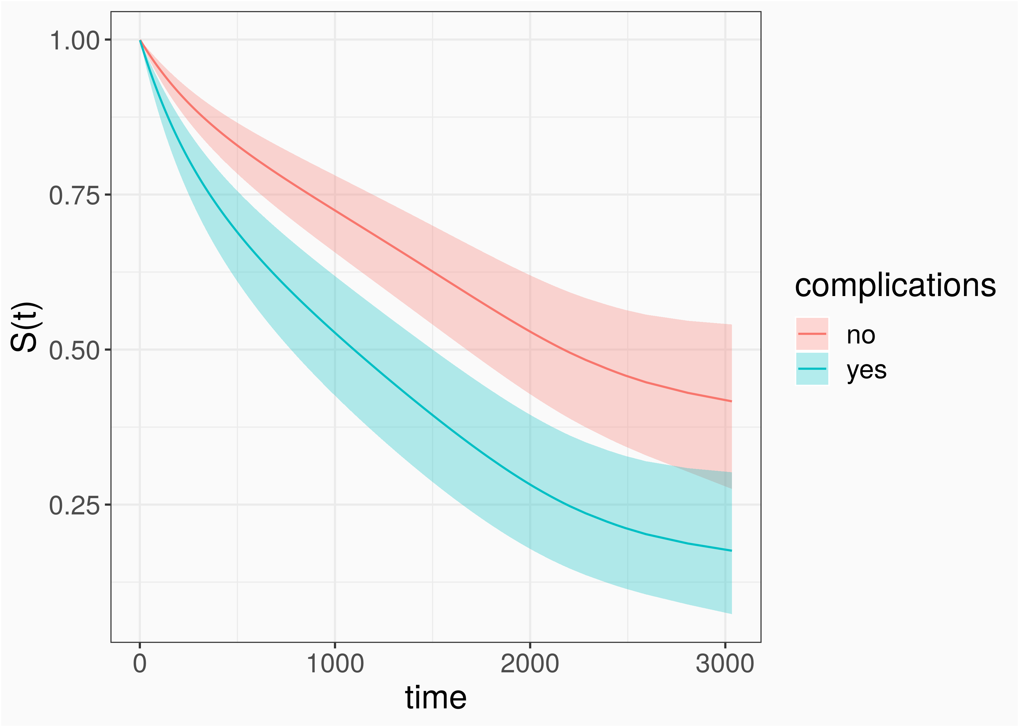
Stratified Model
pam2 <- pamm( formula = ped_status ~ s(tend, by = complications) + sex + s(age), data = ped)summary(pam2)## Parametric coefficients:## Estimate Std. Error z value Pr(>|z|)## (Intercept) -7.78558 0.07921 -98.288 <2e-16 ***## sexfemale 0.15409 0.10584 1.456 0.145## ---## Signif. codes: 0 '***' 0.001 '**' 0.01 '*' 0.05 '.' 0.1 ' ' 1#### Approximate significance of smooth terms:## edf Ref.df Chi.sq p-value## s(tend):complicationsno 6.102 7.279 8.717 0.293## s(tend):complicationsyes 6.096 7.224 126.152 < 2e-16 ***## s(age) 1.051 1.101 23.819 1.6e-06 ***...Stratified Model (Hazard)
gg_slice(ped, pam2, term = "tend", tend = seq(0,1000, by = 10), complications = unique(complications))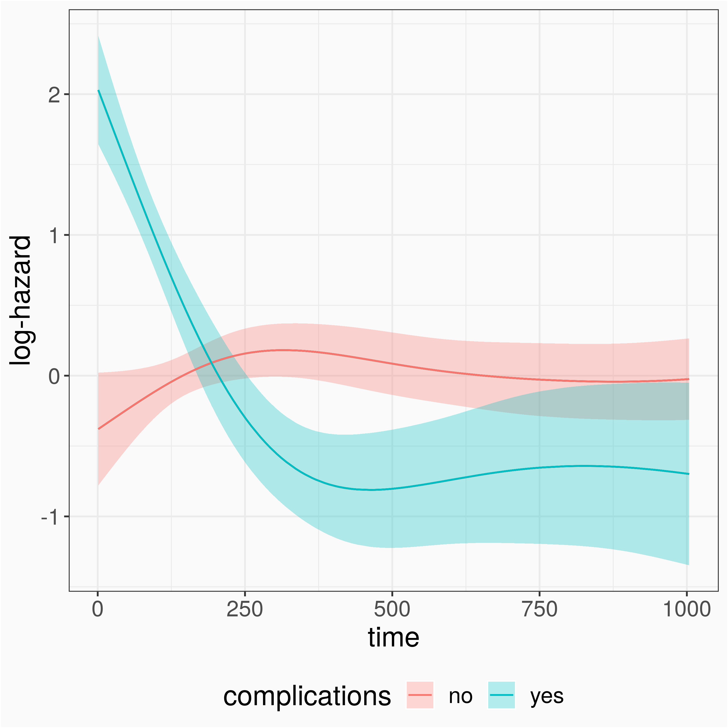
References
Bender, A. et al. (2018). "A generalized additive model approach to time-to-event analysis". En. In: Statistical Modelling 18.3-4, pp. 299-321. ISSN: 1471-082X. DOI: 10.1177/1471082X17748083.
Bender, A. et al. (2020). "A General Machine Learning Framework for Survival Analysis". In: arXiv:2006.15442 [cs, stat]. arXiv: 2006.15442.
Cai, T. et al. (2002). "Mixed Model-Based Hazard Estimation". In: Journal of Computational and Graphical Statistics 11.4, pp. 784-798. ISSN: 1061-8600. DOI: 10.1198/106186002862. URL: http://dx.doi.org/10.1198/106186002862 (visited on Jan. 07, 2015).
Friedman, M. (1982). "Piecewise Exponential Models for Survival Data with Covariates". In: The Annals of Statistics 10.1, pp. 101-113. ISSN: 00905364. URL: http://www.jstor.org/stable/2240502.
Laird, N. et al. (1981). "Covariance Analysis of Censored Survival Data Using Log-Linear Analysis Techniques". In: Journal of the American Statistical Association 76.374, pp. 231-240. DOI: 10.2307/2287816. URL: http://www.jstor.org/stable/2287816.
Wood, S. N. (2017). Generalized Additive Models: An Introduction with R. Englisch. 2 Rev ed.. Boca Raton: Chapman & Hall/Crc Texts in Statistical Science. ISBN: 978-1-4987-2833-1.